|
|
|
|
|
|
|
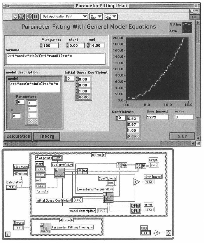
Figure 6.9
The G Math Toolkit allows you to manipulate formulas when you're fitting measured
values while running the program. The model equations, the variable quantity, and
the parameters that occur are fixed (bottom left in the cluster). For easier understanding,
the initial data in the example was also generated using a formula (top of panel).
Additional random terms ensure that you get a true fitting problem. The diagram is
simplicity itself. |
|
|
|
|
|
|
|
|
Kutta, and Cash-Karp, as well as to numeric and symbolic operating routines for systems of linear differential equations and differential equations of the nth order. As an example, let's look at describing the motion of a gyroscope. You can do this by fixing the gyroscope's center of gravity in three-dimensional space (Gander and Hrebicek 1993). There are many parameters that determine the behavior of this system. Figure 6.10 shows the panel of an example VI that displays the equations of motion solved by the G Math Toolkit. |
|
|
|
|
|